Searchlight classification of movie segments

In this analysis, we classify which segment (5 TRs) of the movie the participant was watching for each searchlight (20 mm radius).

Preparations

Import Python packages

import os
import numpy as np
from scipy.stats import ttest_rel, rankdata, pearsonr, spearmanr
import neuroboros as nb
from joblib import Parallel, delayed, cpu_count, parallel_backend

import matplotlib.pyplot as plt
import matplotlib as mpl
import seaborn as sns

Other settings

dsets = ['raiders', 'budapest']
ico = 32
spaces = [f'{a}-ico{b}' for a in ['fsavg', 'fslr', 'onavg'] for b in [ico]]
train_dur, test_dur = '1st-half', '2nd-half'
radius = 20
align_radius = 20
size = 5
colors = np.array(sns.color_palette('tab10'))
np.set_printoptions(4, linewidth=200)
if os.path.exists('Arial.ttf'):
    from matplotlib import font_manager
    font_manager.fontManager.addfont('Arial.ttf')
mpl.rcParams['font.family'] = 'Arial'

Load results

# cache file to avoid excessive I/O
summary_fn = f'sl_clf/summary_ico{ico}_size{size}.pkl'
if not os.path.exists(summary_fn):
    results = {}
    for dset_name in dsets:
        dset = nb.dataset(dset_name)
        sids = dset.subjects
        for align in ['surf', 'procr', 'ridge']:
            for space in spaces:
                folder = f'sl_clf/{dset_name}/{space}_{align}_{align_radius}mm_'\
                    f'{train_dur}_{test_dur}_{size}TRs'
                aa = []
                for sid in sids:
                    a = [np.load(f'{folder}/{sid}_{lr}h_{radius}mm.npy')
                         for lr in 'lr']
                    a = np.concatenate(a)
                    aa.append(a)
                aa = np.array(aa)
                results[dset_name, space, align] = aa
    nb.save(summary_fn, results)
results = nb.load(summary_fn)

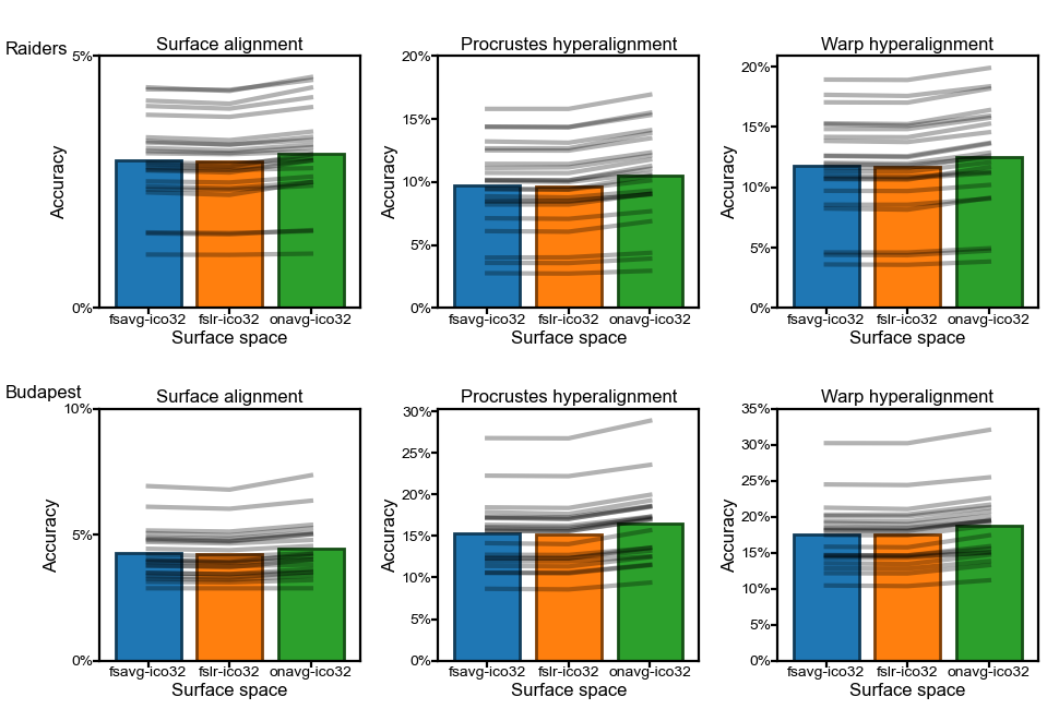
Accuracy of movie time point classification

• Two datasets (top: Raiders, bottom: Budapest)

• Three alignment methods (surface alignment, Procrustes hyperalignment, warp hyperalignment)

• Bars denote average accuracy across participants and searchlights

• Grey lines denote individual participants (average accuracy across searchlights)

fig, axs = plt.subplots(2, 3, figsize=[_/2.54 for _ in (12, 8)], dpi=200)
pct1, pct2, pp = [], [], []
for ii, dset_name in enumerate(['raiders', 'budapest']):
    for jj, align in enumerate(['surf', 'procr', 'ridge']):
        ax = axs[ii, jj]
        ys = []
        for i, space in enumerate(spaces):
            a = results[dset_name, space, align].mean(axis=1)
            m = a.mean(axis=0)
            c = colors[i]
            ax.bar(i, m, facecolor=c, edgecolor=c*0.5, ecolor=c*0.5)
            ys.append(a)
        ax.set_xticks(np.arange(3), labels=spaces)

        ys = np.array(ys)
        for y in ys.T:
            ax.plot(np.arange(3), y, 'k-', alpha=0.3, markersize=1)
        t, p = ttest_rel(ys[2], ys[0])
        pp.append(p)
        assert p < 0.005
        t, p = ttest_rel(ys[2], ys[1])
        pp.append(p)
        assert p < 0.005
        pct1.append(np.mean(ys[0] < ys[2]))
        pct2.append(np.mean(ys[1] < ys[2]))

        max_ = int(np.ceil(ys.max() * 20))
        yy = np.arange(max_ + 1) * 0.05
        ax.set_yticks(yy, labels=[f'{_*100:.0f}%' for _ in yy])
        ax.set_xlim([-0.6, 2.6])
        ax.tick_params(axis='both', pad=0, length=2, labelsize=5)
        ax.set_ylabel('Accuracy', size=6, labelpad=1)
        ax.set_xlabel('Surface space', size=6, labelpad=1)
        title = {'procr': 'Procrustes hyperalignment',
                 'ridge': 'Warp hyperalignment',
                 'surf': 'Surface alignment'}[align]
        ax.set_title(f'{title}', size=6, pad=2)
    ax.annotate(dset_name.capitalize(), (0.005, 0.99 - ii * 0.5),
                xycoords='figure fraction', size=6, va='top')
print(np.mean(pct1), np.mean(pct2), np.max(pp))

fig.subplots_adjust(
    left=0.08, right=0.99, top=0.94, bottom=0.06, wspace=0.3, hspace=0.4)
plt.savefig('sl_clf_bar.png', dpi=300, transparent=True)
plt.show()

1.0 1.0 4.803615811053366e-07

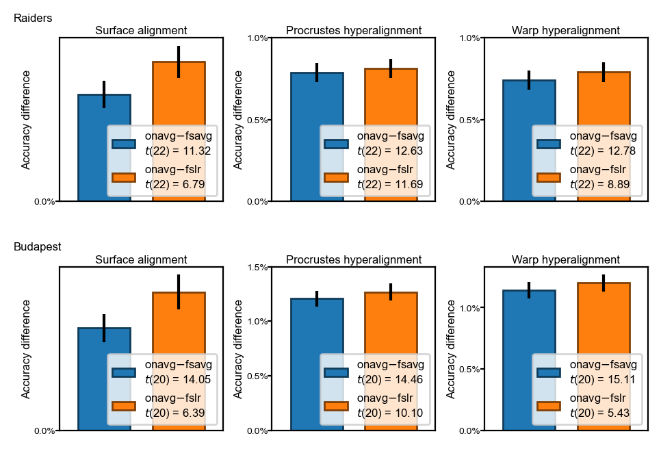
Difference of classification accuracy between template spaces

• The difference accuracy between onavg and fsavg (blue bars), and between onavg and fslr (orange bars)

• The differences are statistically significant (p < 1e-4) across different datasets and alignment methods

fig, axs = plt.subplots(
    2, 3, figsize=[_/2.54 for _ in (12, 8)], dpi=200)
pct1, pct2, pp = [], [], []
for ii, dset_name in enumerate(dsets):
    for jj, align in enumerate(['surf', 'procr', 'ridge']):
        ax = axs[ii, jj]
        max_ = []
        onavg = results[dset_name, spaces[-1], align].mean(axis=1)
        for kk, space in enumerate(spaces[:2]):
            y = onavg - results[dset_name, space, align].mean(axis=1)
            m = y.mean(axis=0)
            se = y.std(axis=0, ddof=1) / np.sqrt(y.shape[0])
            c = colors[kk]
            t, p = ttest_rel(onavg, results[dset_name, space, align][:, -1])
            dof = len(onavg) - 1
            label = f'{spaces[-1].split("-")[0]}$ - ${spaces[kk].split("-")[0]}'\
                    f'\n$t$({dof}) = {t:.2f}'
            ax.bar(kk, m, yerr=se, color=c, ec=c*0.5, width=0.7, label=label)
            max_.append(m + se)
            assert p < 1e-4
        max_ = int(np.ceil(np.max(max_) * 1.1 * 1000))

        ax.set_xticks([])
        ax.set_xlim(np.array([-0.6, 1.6]))
        yy = np.arange(0, max_ + 1, 5)
        ax.set_yticks(yy  * 0.001, labels=[f'{_*0.1:.1f}%' for _ in yy])
        ax.set_ylabel('Accuracy difference', size=6, labelpad=1)
        ax.tick_params(axis='both', pad=0, length=2, labelsize=5)

        title = {'procr': 'Procrustes hyperalignment',
                 'ridge': 'Warp hyperalignment',
                 'surf': 'Surface alignment',
                }[align]
        ax.set_title(f'{title}', size=6, pad=2)
        ax.legend(fontsize=6, fancybox=True, loc='lower right')
    axs[ii, 0].annotate(
        dset_name.capitalize(), (-0.28, 1.15),
        xycoords='axes fraction', size=6, va='top', ha='left')
fig.subplots_adjust(
    left=0.08, right=0.99, top=0.93, bottom=0.02, wspace=0.3, hspace=0.4)
plt.savefig('sl_clf_bar_diff.png', dpi=300, transparent=True)
plt.show()

Which brain region has the most improvement

Upsample the data

• To compare the results based on different template spaces, we upsample the statistics to onavg-ico128 space

upsampled = {}
for ii, dset_name in enumerate(['raiders', 'budapest']):
    for jj, align in enumerate(['surf', 'procr', 'ridge']):
        for space in spaces:
            a = results[dset_name, space, align].mean(axis=0)
            center_space = space.split('-')[0] + '-ico32'
            xfms = [nb.mapping(lr, center_space, 'onavg-ico128', mask=True)
                    for lr in 'lr']
            nv1 = xfms[0].shape[0]
            a = np.concatenate([a[:nv1] @ xfms[0], a[nv1:] @ xfms[1]])
            upsampled[dset_name, space, align] = a

upsampled_ivd = {}
for space in spaces:
    center_space = space.split('-')[0] + '-ico32'
    ivd_lr = []
    for lr in 'lr':
        coords, faces = nb.geometry('midthickness', lr, center_space)
        surf = nb.Surface(coords, faces)
        distances = nb.distances(lr, center_space)
        mask = nb.mask(lr, space=center_space)
        ivd = []
        for i, nbrs in enumerate(surf.neighbors):
            if mask[i]:
                ivd.append(distances[i, nbrs].mean())
        ivd_lr.append(np.array(ivd))

    values = []
    for lr, ivd in zip('lr', ivd_lr):
        sls = nb.sls(lr, radius, space=space)
        avg_ivd = np.array([ivd[sl].mean() for sl in sls])

        xfm = nb.mapping(lr, center_space, 'onavg-ico128', mask=True)
        values.append(avg_ivd @ xfm)
    upsampled_ivd[space] = np.concatenate(values)

Correlations with improvement in accuracy

• Regions that were previously undersampled are more likely to have more improvement after switching to onavg (pearsonr(c, d) in the code below).

• Regions that have higher accuracies based on traditional templates are more likely to have more improvement after switching to onavg (pearsonr(a, d) in the code below).

for space in spaces[:2]:
    for ii, dset_name in enumerate(['raiders', 'budapest']):
        for jj, align in enumerate(['surf', 'procr', 'ridge']):
            a = upsampled[dset_name, space, align]
            b = upsampled[dset_name, spaces[-1], align]
            c = upsampled_ivd[space]
            d = b - a
            print(f'{space:11s}, {dset_name:8s}, {align:5s}, '
                  f'{pearsonr(c, d)[0]:7.4f}, {pearsonr(a, d)[0]:7.4f}')

fsavg-ico32, raiders , surf , -0.0902, -0.0007
fsavg-ico32, raiders , procr,  0.2385,  0.4536
fsavg-ico32, raiders , ridge,  0.4063,  0.4944
fsavg-ico32, budapest, surf , -0.1182, -0.0443
fsavg-ico32, budapest, procr,  0.2056,  0.3686
fsavg-ico32, budapest, ridge,  0.4501,  0.3976
fslr-ico32 , raiders , surf , -0.1038,  0.0102
fslr-ico32 , raiders , procr,  0.2697,  0.4402
fslr-ico32 , raiders , ridge,  0.4472,  0.5102
fslr-ico32 , budapest, surf , -0.0832,  0.0718
fslr-ico32 , budapest, procr,  0.2601,  0.3916
fslr-ico32 , budapest, ridge,  0.4820,  0.4256

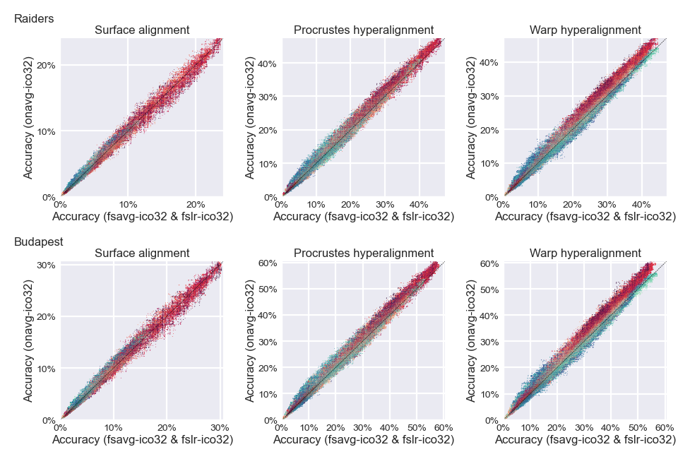
Scatter plots

nc = 10
colors2 = np.concatenate(
    [sns.color_palette("mako", nc)[1:],
     [[0.9, 0.9, 0.9]],
     sns.color_palette("rocket", nc)[1:][::-1]],
    axis=0)
cmap = mpl.colors.LinearSegmentedColormap.from_list('mako_rocket', colors2)

In the figure below, red dots are searchlights that have larger inter-vertex distance based on traditional templates, and blue dots are those that lave smaller inter-vertex distance. Dots above the diagonal are searchlights that improve after switching to onavg, and red dots appear more often above the diagonal.

with sns.axes_style('darkgrid'):
    fig, axs = plt.subplots(2, 3, figsize=[_/2.54 for _ in (12, 8)], dpi=200)
    for ii, dset_name in enumerate(['raiders', 'budapest']):
        for jj, align in enumerate(['surf', 'procr', 'ridge']):
            aa, bb, cc = [], [], []
            for space in spaces[:2]:
                a = upsampled[dset_name, space, align]
                b = upsampled[dset_name, spaces[-1], align]
                c = upsampled_ivd[space]
                aa.append(a)
                bb.append(b)
                cc.append(c)
            aa = np.concatenate(aa)
            bb = np.concatenate(bb)
            cc = np.concatenate(cc)
            cc = cc - np.median(cc)
            vmax = np.percentile(cc, [99])
            idx = np.argsort(bb - aa)
            aa, bb, cc = aa[idx], bb[idx], cc[idx]
            ax = axs[ii, jj]
            ax.scatter(aa, bb, c=cc, s=0.1, edgecolor='none',
                       cmap=cmap, vmin=-vmax, vmax=vmax)
            lim = [0, max(a.max(), b.max())]
            ticks = np.arange(0, np.ceil(lim[1] * 100) + 1, 10) * 0.01
            labels = [f'{_*100:.0f}%' for _ in ticks]
            ax.set_xticks(ticks, labels=labels)
            ax.set_yticks(ticks, labels=labels)
            ax.set_xlim(lim)
            ax.set_ylim(lim)
            ax.plot(lim, lim, 'k--', alpha=1, lw=0.2)
            ax.tick_params(axis='both', pad=0, length=2, labelsize=5)
            ax.set_ylabel(f'Accuracy ({spaces[-1]})', size=6, labelpad=1)
            ax.set_xlabel(f'Accuracy ({" & ".join(spaces[:-1])})',
                          size=6, labelpad=1)
            title = {'procr': 'Procrustes hyperalignment',
                     'ridge': 'Warp hyperalignment',
                     'surf': 'Surface alignment',
                    }[align]
            ax.set_title(f'{title}', size=6, pad=2)
        axs[ii, 0].annotate(
            dset_name.capitalize(), (-0.28, 1.15),
            xycoords='axes fraction', size=6, va='top', ha='left')
    fig.subplots_adjust(
        left=0.08, right=0.99, top=0.92, bottom=0.06, wspace=0.35, hspace=0.4)
    plt.savefig('sl_clf_scatter.png', dpi=300)
    plt.show()