Different data resolutions

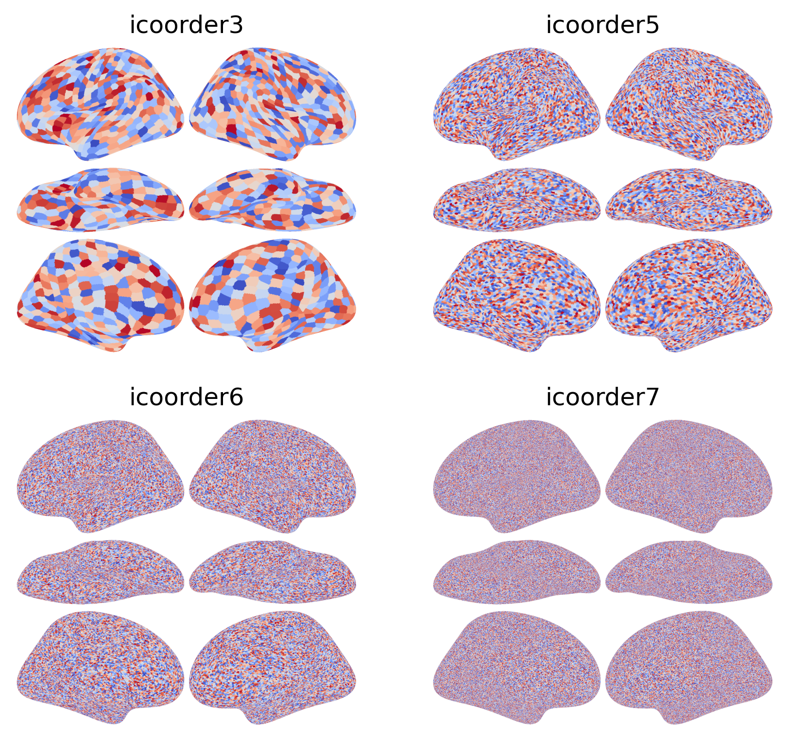
This example is about different input data resolutions.

Neuroimaging data on cortical surface has different spatial resolutions:

name	resolution	# of vertices per hemishere
icoorder7	0.7 mm	163842
icoorder6	1.5 mm	40962
icoorder5	3 mm	10242
icoorder4	6 mm	2562
icoorder3	13 mm	642

Typical the data resolution is between icoorder7 (usually anatomical scans) and icoorder5 (usually functional scans). icoorder3 resolution is often used in defining connectivity targets for connectivity hyperalignment and in examples.

The number of cortical vertices per hemisphere can be computed based on icoorder: \( n_v = 4^{icoorder} \times 10 + 2 \), where \(n_v\) is the number of vertices.

The brain_plot function automatically handles various data resolution between icoorder7 and icoorder3. When the input data has a lower resolution than icoorder7, it’s automatically upsampled to the icoorder7 resolution in a nearest-neighbor manner based on the Voronoi diagram. The data is always visualized using the icoorder7 high-resolution surface (i.e., fsaverage).

import numpy as np
from brainplotlib import brain_plot
import matplotlib.pyplot as plt

rng = np.random.default_rng(0)

fig, axs = plt.subplots(2, 2, dpi=300, figsize=([_/300 + 1 for _ in [1728, 1560]]))
icoorders = [3, 5, 6, 7]
for i in range(2):
    for j in range(2):
        ax = axs[i][j]
        icoorder = icoorders[i*2+j]
        nv = 4**icoorder * 10 + 2
        v = rng.random((nv * 2, ))
        img = brain_plot(v, vmax=1, vmin=0, cmap='coolwarm')
        ax.imshow(img)
        ax.axis('off')
        ax.set_title(f'icoorder{icoorder}')
plt.show()

---

<< Go back to the gallery of examples